Plot expected and actual mean spending per transaction

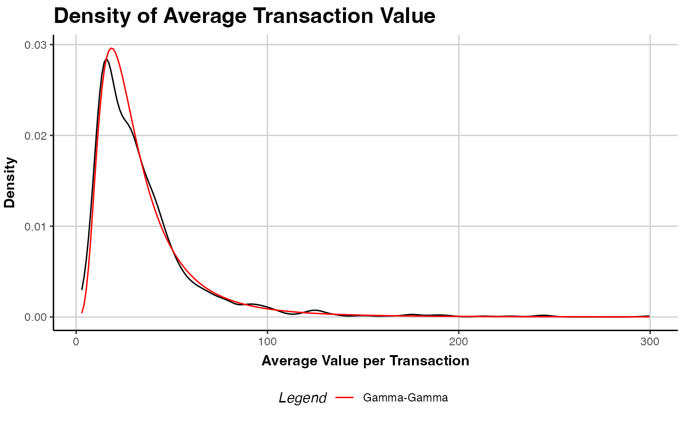
Compares the density of the observed average spending per transaction (empirical distribution) to the model's distribution of mean transaction spending (weighted by the actual number of transactions). See plot.clv.data to plot more nuanced diagnostics for the transaction data only.

# S3 method for clv.fitted.spending
plot(x, n = 256, verbose = TRUE, ...)

# S4 method for clv.fitted.spending
plot(x, n = 256, verbose = TRUE, ...)

Arguments

x

The fitted spending model to plot

n

Number of points at which the empirical and model density are calculated. Should be a power of two.

verbose

Show details about the running of the function.

...

Ignored

Value

An object of class ggplot from package ggplot2 is returned by default.

References

Colombo R, Jiang W (1999). “A stochastic RFM model.” Journal of Interactive Marketing, 13(3), 2-12.

Fader PS, Hardie BG, Lee K (2005). “RFM and CLV: Using Iso-Value Curves for Customer Base Analysis.” Journal of Marketing Research, 42(4), 415-430.

Fader PS, Hardie BG (2013). “The Gamma-Gamma Model of Monetary Value.” URL http://www.brucehardie.com/notes/025/gamma_gamma.pdf.

See also

plot for transaction models

plot for transaction diagnostics of clv.data objects

Examples

# \donttest{
data("cdnow")

clv.cdnow <- clvdata(cdnow,
  date.format="ymd",
  time.unit = "week",
  estimation.split = "1997-09-30")

est.gg <- gg(clv.data = clv.cdnow)
#> Starting estimation...
#> Estimation finished!

# Compare empirical to theoretical distribution
plot(est.gg)


if (FALSE) {
# Modify the created plot further
library(ggplot2)
gg.cdnow <- plot(est.gg)
gg.cdnow + ggtitle("CDnow Spending Distribution")
}
# }