Fits the Gamma-Gamma model on a given object of class clv.data to predict customers' mean
spending per transaction.
Arguments
- clv.data
The data object on which the model is fitted.
- start.params.model
Named start parameters containing the optimization start parameters for the model without covariates.
- remove.first.transaction
Whether customer's first transaction are removed. If
TRUEall zero-repeaters are excluded from model fitting.- optimx.args
Additional arguments to control the optimization which are forwarded to
optimx::optimx. If multiple optimization methods are specified, only the result of the last method is further processed.- verbose
Show details about the running of the function.
- ...
Ignored
Value
An object of class clv.gg is returned.
The function summary can be used to obtain and print a summary of the results.
The generic accessor functions coefficients, vcov, fitted,
logLik, AIC, BIC, and nobs are available.
Details
Model parameters for the G/G model are p, q, and gamma. p: shape parameter of the Gamma distribution of the spending process. q: shape parameter of the Gamma distribution to account for customer heterogeneity. gamma: scale parameter of the Gamma distribution to account for customer heterogeneity.
If no start parameters are given, p=0.5, q=15, gamma=2 is used for all model parameters. All parameters are required
to be > 0.
The Gamma-Gamma model cannot be estimated for data that contains negative prices. Customers with a mean spending of zero or a transaction count of zero are ignored during model fitting.
References
Colombo R, Jiang W (1999). “A stochastic RFM model.” Journal of Interactive Marketing, 13(3), 2-12.
Fader PS, Hardie BG, Lee K (2005). “RFM and CLV: Using Iso-Value Curves for Customer Base Analysis.” Journal of Marketing Research, 42(4), 415-430.
Fader PS, Hardie BG (2013). “The Gamma-Gamma Model of Monetary Value.” URL http://www.brucehardie.com/notes/025/gamma_gamma.pdf.
See also
Examples
# \donttest{
data("apparelTrans")
clv.data.apparel <- clvdata(apparelTrans, date.format = "ymd",
time.unit = "w", estimation.split = 52)
# Fit the gg model
gg(clv.data.apparel)
#> Starting estimation...
#> Estimation finished!
#> Gamma-Gamma Model
#>
#> Call:
#> gg(clv.data = clv.data.apparel)
#>
#> Coefficients:
#> p q gamma
#> 4.090 4.162 28.705
#> KKT1: TRUE
#> KKT2: TRUE
# Give initial guesses for the model parameters
gg(clv.data.apparel,
start.params.model = c(p=0.5, q=15, gamma=2))
#> Starting estimation...
#> Estimation finished!
#> Gamma-Gamma Model
#>
#> Call:
#> gg(clv.data = clv.data.apparel, start.params.model = c(p = 0.5,
#> q = 15, gamma = 2))
#>
#> Coefficients:
#> p q gamma
#> 4.090 4.163 28.707
#> KKT1: TRUE
#> KKT2: TRUE
# pass additional parameters to the optimizer (optimx)
# Use Nelder-Mead as optimization method and print
# detailed information about the optimization process
apparel.gg <- gg(clv.data.apparel,
optimx.args = list(method="Nelder-Mead",
control=list(trace=6)))
#> Starting estimation...
#> fn is fn1
#> Looking for method = Nelder-Mead
#> Methods to be used:[1] "Nelder-Mead"
#> optcfg:$fname
#> [1] "fn1"
#>
#> $npar
#> [1] 3
#>
#> $ctrl
#> $ctrl$follow.on
#> [1] FALSE
#>
#> $ctrl$save.failures
#> [1] TRUE
#>
#> $ctrl$trace
#> [1] 6
#>
#> $ctrl$kkt
#> [1] TRUE
#>
#> $ctrl$all.methods
#> [1] FALSE
#>
#> $ctrl$starttests
#> [1] FALSE
#>
#> $ctrl$maximize
#> [1] FALSE
#>
#> $ctrl$dowarn
#> [1] TRUE
#>
#> $ctrl$usenumDeriv
#> [1] FALSE
#>
#> $ctrl$kkttol
#> [1] 0.001
#>
#> $ctrl$kkt2tol
#> [1] 1e-06
#>
#> $ctrl$badval
#> [1] 8.988466e+307
#>
#> $ctrl$scaletol
#> [1] 3
#>
#> $ctrl$have.bounds
#> [1] FALSE
#>
#>
#> $usenumDeriv
#> [1] FALSE
#>
#> $ufn
#> function (par)
#> fn(par, ...)
#> <bytecode: 0x10cb449e0>
#> <environment: 0x11e4f7070>
#>
#> $have.bounds
#> [1] FALSE
#>
#> $method
#> [1] "Nelder-Mead"
#>
#> Method: Nelder-Mead
#> Nelder-Mead direct search function minimizer
#> function value for initial parameters = 2320.550547
#> Scaled convergence tolerance is 3.45789e-05
#> Stepsize computed as 0.100000
#> BUILD 4 2413.593778 2287.962766
#> EXTENSION 6 2320.550547 2118.179626
#> LO-REDUCTION 8 2288.939380 2118.179626
#> EXTENSION 10 2287.962766 2006.752787
#> EXTENSION 12 2140.779908 1865.377077
#> LO-REDUCTION 14 2118.179626 1865.377077
#> EXTENSION 16 2006.752787 1816.029388
#> LO-REDUCTION 18 1879.017352 1814.392354
#> LO-REDUCTION 20 1865.377077 1811.105613
#> HI-REDUCTION 22 1816.724761 1811.105613
#> HI-REDUCTION 24 1816.029388 1810.011973
#> HI-REDUCTION 26 1814.392354 1810.011973
#> EXTENSION 28 1812.328256 1803.967207
#> EXTENSION 30 1811.105613 1797.448167
#> EXTENSION 32 1810.011973 1792.651448
#> EXTENSION 34 1803.967207 1771.069003
#> LO-REDUCTION 36 1797.448167 1771.069003
#> EXTENSION 38 1792.651448 1736.929680
#> EXTENSION 40 1774.316285 1696.379972
#> LO-REDUCTION 42 1771.069003 1696.379972
#> EXTENSION 44 1736.929680 1594.842593
#> LO-REDUCTION 46 1705.673499 1594.842593
#> EXTENSION 48 1696.379972 1543.163720
#> LO-REDUCTION 50 1648.521091 1543.163720
#> REFLECTION 52 1594.842593 1504.492492
#> HI-REDUCTION 54 1556.787712 1504.492492
#> LO-REDUCTION 56 1549.465591 1504.492492
#> LO-REDUCTION 58 1543.163720 1504.492492
#> LO-REDUCTION 60 1533.857044 1504.492492
#> LO-REDUCTION 62 1511.527117 1504.492492
#> LO-REDUCTION 64 1507.812361 1503.645411
#> HI-REDUCTION 66 1507.121621 1503.645411
#> HI-REDUCTION 68 1504.804163 1503.645411
#> LO-REDUCTION 70 1504.492492 1503.645411
#> HI-REDUCTION 72 1504.385094 1503.645411
#> HI-REDUCTION 74 1504.004887 1503.645411
#> LO-REDUCTION 76 1503.924113 1503.645411
#> LO-REDUCTION 78 1503.871791 1503.645411
#> REFLECTION 80 1503.733127 1503.580032
#> REFLECTION 82 1503.656945 1503.529114
#> HI-REDUCTION 84 1503.645411 1503.529114
#> EXTENSION 86 1503.580032 1503.317265
#> LO-REDUCTION 88 1503.574968 1503.317265
#> EXTENSION 90 1503.529114 1503.187812
#> EXTENSION 92 1503.446600 1502.825206
#> EXTENSION 94 1503.317265 1502.503977
#> EXTENSION 96 1503.187812 1501.883004
#> EXTENSION 98 1502.825206 1500.833335
#> LO-REDUCTION 100 1502.503977 1500.833335
#> EXTENSION 102 1501.883004 1498.679882
#> LO-REDUCTION 104 1500.908856 1498.679882
#> EXTENSION 106 1500.833335 1498.025422
#> HI-REDUCTION 108 1499.273672 1498.025422
#> LO-REDUCTION 110 1499.196113 1498.025422
#> EXTENSION 112 1498.679882 1496.488212
#> HI-REDUCTION 114 1498.282504 1496.488212
#> EXTENSION 116 1498.025422 1495.480929
#> EXTENSION 118 1497.727222 1494.028696
#> LO-REDUCTION 120 1496.488212 1494.028696
#> EXTENSION 122 1495.480929 1491.004905
#> LO-REDUCTION 124 1494.352549 1491.004905
#> LO-REDUCTION 126 1494.028696 1491.004905
#> REFLECTION 128 1491.568134 1490.419555
#> HI-REDUCTION 130 1491.448804 1490.419555
#> EXTENSION 132 1491.004905 1489.493080
#> LO-REDUCTION 134 1490.912176 1489.493080
#> LO-REDUCTION 136 1490.419555 1489.493080
#> REFLECTION 138 1489.737964 1489.433009
#> LO-REDUCTION 140 1489.547197 1489.387178
#> HI-REDUCTION 142 1489.493080 1489.326166
#> LO-REDUCTION 144 1489.433009 1489.315144
#> LO-REDUCTION 146 1489.387178 1489.315144
#> LO-REDUCTION 148 1489.326166 1489.294595
#> HI-REDUCTION 150 1489.319300 1489.294595
#> REFLECTION 152 1489.315144 1489.273802
#> HI-REDUCTION 154 1489.298973 1489.273802
#> REFLECTION 156 1489.294595 1489.273140
#> HI-REDUCTION 158 1489.283957 1489.273140
#> REFLECTION 160 1489.275274 1489.268652
#> HI-REDUCTION 162 1489.273802 1489.268652
#> REFLECTION 164 1489.273140 1489.267276
#> LO-REDUCTION 166 1489.270088 1489.267276
#> HI-REDUCTION 168 1489.268837 1489.267276
#> LO-REDUCTION 170 1489.268652 1489.267276
#> LO-REDUCTION 172 1489.267993 1489.267276
#> HI-REDUCTION 174 1489.267578 1489.267276
#> LO-REDUCTION 176 1489.267491 1489.267245
#> LO-REDUCTION 178 1489.267381 1489.267163
#> HI-REDUCTION 180 1489.267276 1489.267163
#> HI-REDUCTION 182 1489.267245 1489.267157
#> Exiting from Nelder Mead minimizer
#> 184 function evaluations used
#> Post processing for method Nelder-Mead
#> Successful convergence!
#> Compute Hessian approximation at finish of Nelder-Mead
#> Compute gradient approximation at finish of Nelder-Mead
#> Save results from method Nelder-Mead
#> $par
#> log.p log.q log.gamma
#> 1.409896 1.425674 3.355160
#>
#> $value
#> [1] 1489.267
#>
#> $message
#> NULL
#>
#> $convcode
#> [1] 0
#>
#> $fevals
#> function
#> 184
#>
#> $gevals
#> gradient
#> NA
#>
#> $nitns
#> [1] NA
#>
#> $kkt1
#> [1] TRUE
#>
#> $kkt2
#> [1] TRUE
#>
#> $xtimes
#> user.self
#> 0.015
#>
#> Assemble the answers
#> Estimation finished!
# estimated coefs
coef(apparel.gg)
#> p q gamma
#> 4.095528 4.160661 28.650189
# summary of the fitted model
summary(apparel.gg)
#> Gamma-Gamma Model
#>
#> Call:
#> gg(clv.data = clv.data.apparel, optimx.args = list(method = "Nelder-Mead",
#> control = list(trace = 6)))
#>
#> Fitting period:
#> Estimation start 2005-01-02
#> Estimation end 2006-01-01
#> Estimation length 52.0000 Weeks
#>
#> Coefficients:
#> Estimate Std. Error z-val Pr(>|z|)
#> p 4.0955 0.8965 NA NA
#> q 4.1607 0.5876 NA NA
#> gamma 28.6502 10.2912 NA NA
#>
#> Optimization info:
#> LL -1489.2672
#> AIC 2984.5343
#> BIC 2997.7251
#> KKT 1 TRUE
#> KKT 2 TRUE
#> fevals 184.0000
#> Method Nelder-Mead
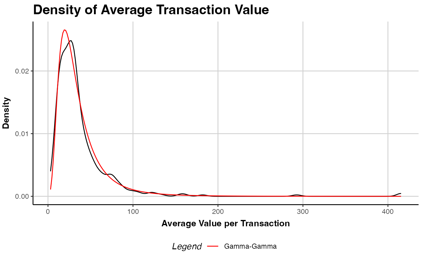
# Plot model vs empirical distribution
plot(apparel.gg)
 # predict mean spending and compare against
# actuals in the holdout period
predict(apparel.gg)
#> Key: <Id>
#> Id actual.mean.spending predicted.mean.spending
#> <char> <num> <num>
#> 1: 1 104.82000 63.80198
#> 2: 10 31.65500 38.10401
#> 3: 100 37.03889 37.12440
#> 4: 101 0.00000 33.08068
#> 5: 102 0.00000 37.12440
#> ---
#> 596: 95 22.76000 28.28877
#> 597: 96 84.53667 37.12440
#> 598: 97 0.00000 37.12440
#> 599: 98 0.00000 34.87553
#> 600: 99 13.99000 16.10190
# }
# predict mean spending and compare against
# actuals in the holdout period
predict(apparel.gg)
#> Key: <Id>
#> Id actual.mean.spending predicted.mean.spending
#> <char> <num> <num>
#> 1: 1 104.82000 63.80198
#> 2: 10 31.65500 38.10401
#> 3: 100 37.03889 37.12440
#> 4: 101 0.00000 33.08068
#> 5: 102 0.00000 37.12440
#> ---
#> 596: 95 22.76000 28.28877
#> 597: 96 84.53667 37.12440
#> 598: 97 0.00000 37.12440
#> 599: 98 0.00000 34.87553
#> 600: 99 13.99000 16.10190
# }